Rotations with Quaternions

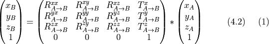
Transformation matrices are an essential component to TF2. They allow for all the different components in a robot to use different reference axes (or frames) and their relationships. A Concise Introduction to Robot Programming with ROS2 (Rico 2023, pg. 65-66) gives a good overview of the general process that TF2 uses:

Algebraically, [relating frames] is done using homogeneous coordinates of a point $P$ in a frame $A$ , this is $P_{A}$ , we can calculate $P_{B}$ in frame $B$ using the transformation matrix $RT_{A \rightarrow B}$ as follows:

$\begin{align} P_{B} &= RT_{A \rightarrow B} * P_{A} & (4.1) \end{align}$

$\begin{align} \begin{pmatrix} x_{B} \\ y_{B} \\ z_{B} \\ 1 \end{pmatrix} &= \begin{pmatrix} R^{xx}_{A \rightarrow B} & R^{xy}_{A \rightarrow B} & R^{xz}_{A \rightarrow B} & T^{x}_{A \rightarrow B} \\ R^{yx}_{A \rightarrow B} & R^{yy}_{A \rightarrow B} & R^{yz}_{A \rightarrow B} & T^{y}_{A \rightarrow B} \\ R^{zx}_{A \rightarrow B} & R^{zy}_{A \rightarrow B} & R^{zz}_{A \rightarrow B} & T^{z}_{A \rightarrow B} \\ 0 & 0 & 0 & 1\end{pmatrix} * \begin{pmatrix} x_{A} \\ y_{A} \\ z_{A} \\ 1 \end{pmatrix} & (4.2) \end{align}$

TF2 uses messages of type tf2_msgs/msg/TFMessage, which holds the following data:

$ ros2 interface show tf2_msgs/msg/TFMessage

geometry_msgs/TransformStamped[] transforms
    std_msgs/Header header
    string child_frame_id
    Transform transform
        Vector3 translation
            float64 x
            float64 y
            float64 z
        Quaternion rotation
            float64 x 0
            float64 y 0
            float64 z 0
            float64 w 1

As transformations are propagated through a system’s TF tree, it is standard for the output header to match the input header. The child frame ID is the ID of the new frame to be created by a given transformation.

The transform itself consists of a translation and a rotation. The translation describes the Euclidean distance between the “origin” of each frame. For example, this could be the distance from the robot’s center to the center of one of its sensors. The rotation describes how the frame is rotated after the translation is applied. For example, two of RoboFlock’s ultrasonic sensor’s do not face the same direction as the robot’s “forward” direction, so a rotation would need to be applied.

This message definition contains an interesting term: quaternion. Quaternions are mathematical objects used to described 3D orientations and rotations. From Quaternions: Theory and Applications (Griffin 2017, pg.88-89):

[The] attitude of a rigid body can be represented by unit quaternion, consisting of a unit vector $\vec{e}$ known as the Euler axis, and a rotation angle $\beta$ about this axis. The quaternion $q$ is the defined as follows:

$\begin{align} q &= \begin{pmatrix} \cos \frac{\beta}{2} \\ \vec{e} \sin \frac{\beta}{2} \end{pmatrix} = \begin{pmatrix} q_{0} \\ \vec{q} \end{pmatrix} \in \mathbb{H} & (1) \end{align}$

where

$\begin{align} \mathbb{H} &= \ \ \begin{array}{ll} \qquad \ \{ \ q \ | \ q_{0}^{2} + \vec{q}^{\ T} \ \vec{q} = 1 \\ q = [ \ q_{0} \ \vec{q}^{\ T} \ ]^{\ T}, \ q_{0} \in \mathbb{R}, \ \vec{q} \in \mathbb{R}^{3} \ \} \end{array} & (2) \end{align}$

$\vec{q} = [q_{1} \ q_{2} \ q_{3}]^{T}$ and $q_{0}$ are known as the vector and scalar parts of the quaternion respectively. In attitude control applications, the unit quaternion represents the rotation from an inertial coordinate systen $N(x_{n}, \ y_{n}, \ z_{n})$ located at some point in the space (for instance, the earth NED frame), to the body coordinate system $B(x_{b}, \ y_{b}, \ z_{b})$ located on the center of mass of a rigid body.

If $\vec{r}$ is a vector expressed in $N$ , then its coordinates in $B$ are expressed by:

$\begin{align} b &= \overline{q} \otimes r \otimes q & (3) \end{align}$

where $b = [0 \ \vec{b}^{\ T}]^{T}$ and $r = [0 \ \vec{r}^{\ T}]^{T}$ are the quaternions associated to vectors $\vec{b}$ and $\vec{r}$ respectively. $\otimes$ denotes the quaternion multiplication and $\overline{q}$ is the conjugate quaternion multiplication of $q$ , defined as:

$\begin{align} \overline{q} &= [q_{0} - \vec{q}^{\ T}]^{T} & (4) \end{align}$

The rotation matrix $C(q)$ corresponding to the attitude quaternion $q$ , is computed as:

$\begin{align} C(q) &= (q_{0}^{2} - \vec{q}^{\ T} \ \vec{q})I_{3} + 2(\vec{q} \vec{q}^{\ T} - q_{0} [\vec{q}^{x}]) & (5) \end{align}$

where $I_{3}$ is the identity matrix and $[\xi^{x}]$ is a skew symmetric tensor associated with the axis vector $\xi$ :

$\begin{align} [\xi^{x}] &= \begin{pmatrix} \xi_{1} \\ \xi_{2} \\ \xi_{3} \end{pmatrix}^{x} = \begin{pmatrix} 0 & -\xi_{3} & \xi_{2} \\ \xi_{3} & 0 & -\xi_{1} \\ -\xi_{2} & \xi_{1} & 0 \end{pmatrix} & (6) \end{align}$

Thus, the coordinate of vector $\vec{r}$ expressed in the $B$ frame is given by:

$\begin{align} \vec{b} &= C(q)\vec{r} & (7) \end{align}$

Let’s break this down, one equation at a time:

The Quaternion Definition

A quaternion $q$ can also be described by $a + b \hat{\imath} + c \hat{\jmath} + d \hat{k}; \ a, b, c, d \in \mathbb{R}$ with $a$ being its rotational scalar and $b, c, d$ being the coefficients of its basis vectors. We can also visualize this as a $4 \times 1$ column vector, but we’ll use the given coefficients instead of $a,b,c,d$ :

$\begin{pmatrix} \cos \frac{\beta}{2} \\ e_{1} \sin \frac{\beta}{2} \\ e_{2} \sin \frac{\beta}{2} \\ e_{3} \sin \frac{\beta}{2} \end{pmatrix}$

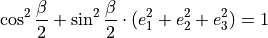
The Set of All Quaternions

We can think of $q_{0}^{2} + \vec{q}^{T} \vec{q} = 1$ in a similar way as the definition of a unit circle, $x^{2} + y^{2} = 1$ . Remember that the dot prouct $\vec{q}^{T} \vec{q}$ (which is equivalent to $\vec{q} \vec{q}^{T}$ ) produces a scalar value. If we expand this notation out, our equation looks like this:

$\cos^{2} \frac{\beta}{2} + \sin^{2} \frac{\beta}{2} \cdot (e_{1}^{2} + e_{2}^{2} + e_{3}^{2}) = 1$

The other rule, $q = [q_{0} \vec{q}^{T}]^{T}$ , simply means that the quaternion $q$ is a column vector in which the first entry is the rotational scalar $q_{0}$ , and the following three entries corresponding to quaternion’s 3D vector.

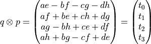
Quaternion Multiplication

Quaternion multiplication is a non-commutative (i.e., order matters) operation that essentially applies each quaternion’s rotation in succession. Consider quaternions $q = [a b c d]^{T}$ and $p = [e f g h]^{T}$ . We define their product, $t$ , as follows:

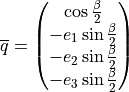
$q \otimes p = \begin{pmatrix} ae - bf - cg -dh \\ af + be + ch + dg \\ ag - bh + ce + df \\ ah + bg - cf + de \end{pmatrix} = \begin{pmatrix} t_{0} \\ t_{1} \\ t_{2} \\ t_{3} \end{pmatrix}$

Conjugate Quaternion Multiplication

Here we refer to the quaternion’s conjugate, which is obtained by negating each of the vector’s entries, effectively inverting the direction of the quaternion’s vector component. In our case, the conjugate is:

$\overline{q} = \begin{pmatrix} \cos \frac{\beta}{2} \\ -e_{1} \sin \frac{\beta}{2} \\ -e_{2} \sin \frac{\beta}{2} \\ -e_{3} \sin \frac{\beta}{2} \end{pmatrix}$

Rotation Matrices

Rotation matrices are use in matrix multiplication with column vectors to enact some rotation in the vector’s plane by some angle. Here, we are given the rotation matrix $C(q)$ that is made up of four components:

$q_{0}^{2} - \vec{q}^{\ T} \vec{q}$ results in an arbitrary scalar value that we’ll denote as $\omega$ .

$I_{3}$ is the $3 \times 3$ identity matrix, i.e., its diagonal entries are all 1 and all other entries are 0.

$\vec{q} \ \vec{q}^{\ T}$ is the dot product between the quaternion’s vector component and itself, which we will denote as $\alpha$ .

$[\vec{q}^{\ x}]$ is a skew symmetric tensor with axis vector $\vec{q}$ .

Note

Tensors are a whole discussion of their own, so we won’t go into depth about them, but here’s a broad overview:

Tensors are algebraic objects that describe multilinear relationships (i.e., relationships between multiple linear variables) between sets of algebraic objects associated with a vector space, such as vectors, scalars, matrices, and other tensors.
Skew-symmetric tensors are tensors whose components change signs when any two indices are swapped, i.e., for some tensor $T$ , we have $T^{T} = -T$ .

Given each of these components, the resulting rotation matrix should look like:

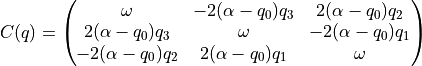
$C(q) = \begin{pmatrix} \omega & -2(\alpha - q_{0})q_{3} & 2(\alpha - q_{0})q_{2} \\ 2(\alpha - q_{0})q_{3} & \omega & -2(\alpha - q_{0})q_{1} \\ -2(\alpha - q_{0})q_{2} & 2(\alpha - q_{0})q_{1} & \omega \end{pmatrix}$

Notice the symmetry between the columns and the rows. Each axis moves in its own plane by the scalar $\omega$ . In the remaining two planes, the axis moves by the scalar $(\alpha - q_{0})$ times the respective vector component $q_{i}$ . This is how quaternions end up describing 3D rotations! The rotation angle $\beta$ , which controls the value of $q_{0}$ , ultimately decides how a quaternion acts on a 3D object.

In the context of ROS2, we can think of our odom frame as being the Euler axis, $\vec{e}$ . Describing our translations between frames is essentially defining a value of $\beta$ that can enact the necessary rotations between any two frames. By setting up the relationships between frames, we are giving TF2 the information it needs to use dynamic translations that update as the robot moves around. In other words, TF2 gives the robot a sense of its surroundings.

References

Griffin, S. (Ed.). (2017). Quaternions : Theory and applications. Nova Science Publishers, Incorporated.

Rico, F. (2023). A Concise Introduction to Robot Programming with ROS2. CRC Press.